It has been a few years since my last post with a list of ten great R functions. Accordingly, it is about time to share yet another ten great R functions. Some of the functions are old, some are new. Some of the functions will (or should) be of interest to most R users, other functions will only be of interest to a small group of people.
See these functions as recommendations for functions to use in R in 2024, similar to how my first post in the series provided recommendations for functions to use in 2021. I believe the previous posts are still full of great recommendations, but you never know. Use R functions at your own discretion.
21. reprex::reprex()
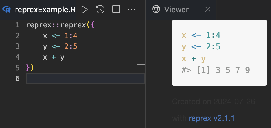
When you collaborate with colleagues, you often have to share both code and results. For this particular task, I find the function reprex() from the package {reprex} extremely useful. Here is an example:
reprex::reprex({
    x <- 1:4
    y <- 2:5
    x + y
})
Here is what it looks like in practice:

Of course, this function is useful in cases where you have to share code, also if you have to ask for help or if you have to share code in a blog post (like this one). Use it to make reproducible examples of your code when you share it with your peers.
22. data.table::let()
I have used {data.table} a lot as of late, and it is growing on me. I would even go as far as to call it my favourite package today. It is highly efficient when working with data frames with millions of rows, and I have used the package several times a week for a long time now.
The one operator in the package I do not really enjoy is :=, especially when used to manipulate multiple variables with `:=`(). Luckily, {data.table} v1.15.0 introduced the function let() that makes it a lot easier to create variables (similar to the let variable binding in other programming languages, such as JavaScript and Rust).
Below is a simple example where we first create a data.table called mtcarsDT before we use let() to create a variable called cylDif with the difference in cyl to the median cyl value.
library("data.table")

mtcarsDT <- as.data.table(mtcars)

mtcarsDT[, let(cylDif = cyl - median(cyl))]

mtcarsDT[1:4, .(cyl, cylDif)]
#>      cyl cylDif
#>    <num>  <num>
#> 1:     6      0
#> 2:     6      0
#> 3:     4     -2
#> 4:     6      0
The {data.table} package has seen a lot of interesting developments over the years, and I can only recommend checking it out, especially if you work with larger datasets in R. If you are mostly familiar with base R or/and tidyverse, just make sure that you actually understand what is going on in the working memory, e.g., when to remember to use data.table::copy().
23. renv::init()
This is more of a package recommendation than a particular function. The {renv} package makes it easy to create a reproducible environment for an R project, and in particular to make sure that a project is reproducible with the version of R and the packages being used, basically bringing the venv experience in Python to R.
The init() function in the package initiates using renv in the current project. It is relatively easy to get started with renv (see, e.g., the introduction to renv), and while it is not as straightforward as venv in Python, it is worth considering it. It can also be used in combination with Docker (which I can highly recommend if you are working with Shiny apps).
Do also check out this good tutorial on how to work with renv for R and Python.
24. directlabels::geom_dl()
One of the functions I did not include in my post with tips and tricks for ggplot2 was directlabels::geom_dl(). However, as it is one of the functions I rely on a lot in my data visualisations, it deserves a plug.
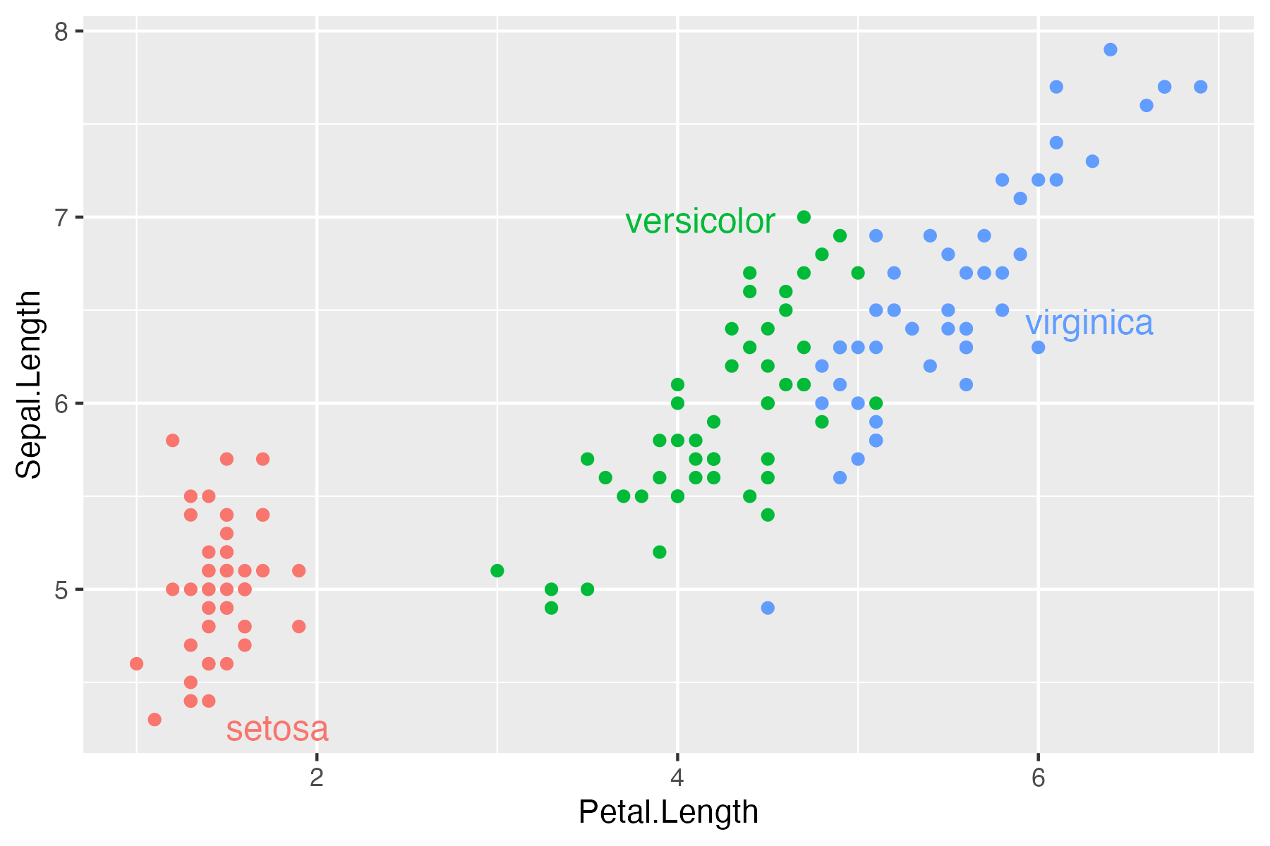
In brief, the function makes it easy to provide direct labels on your plot, i.e., labels much closer to the actual data instead of the separate legend/key. Here is a modified relevant example from the documentation of the package (assuming that you already have {ggplot2} in your environment):
iris |>
    ggplot(aes(x = Petal.Length, y = Sepal.Length,
               label = Species, colour = Species)) +
    geom_point() +
    directlabels::geom_dl(method = "smart.grid") +
    theme(legend.position = "none")

As always, I can recommend checking out the repository awesome-ggplot2 for great packages and guides related to {ggplot2}.
25. beepr::beep()
A lot of the I execute in R takes more than 60 seconds to run. In those cases, it is not optimal to manually check whether R is done or not. Instead, it is good to insert a bit of code at the end of your script that will play a sound when the code is done. To this end, I can recommend {beepr}.
The idea of beepr::beep() is simple: once you run it, it plays a beep. However, it comes with several different sounds in the package. For example, it can play the ‘work complete’ sound from Warcraft II:
beepr::beep(sound = "complete")
Or the ‘stage clear’ sound from Super Mario:
beepr::beep(sound = "mario")
For an overview of all sounds included in the package, check out the associated GitHub page.
26. janitor::excel_numeric_to_date()
If you import a lot of data into R from Excel files, you might have encountered issues with dates (among other issues). For example, instead of dates, you might get a series of number. Luckily, the function excel_numeric_to_date() from the {janitor} package is useful when converting numbers to dates.
janitor::excel_numeric_to_date(35000)
#> [1] "1995-10-28"
To make matters a bit annoying, you will need to ensure that you check the date encoding system of Excel, and do check out the documentation for the function before using it.
27. lintr::lint()
When I share code with colleagues for code review (or for any other purpose), I make sure that my code follows a coherent style with no obvious errors or issues. To do this, I rely on the package {lintr}. The package provides so-called static code analysis for R and will let you know where in your script you have issues (and what the issues are).
See the package website for more information. You can find my current lintr config here.
28. DBI::dbConnect()
I have previously written about using SQL and R together. In the same way that we tend to focus more on the analysis of data and less on data wrangling, we also tend to not focus a lot – if at all – on getting data into R.
I cannot imagine a world without DBI::dbConnect(). Sure, if it did not exist, somebody would (hopefully) create a similar function, but that is beyond the point. If you want to connect to a DBMS, DBI::dbConnect() is the best function in town. Do check out the reference manual for an overview of methods in other packages that can be used in the function.
Also, talking about SQL in R, it is good to also plug the glue_sql() function in {glue}. If you use paste() for SQL queries, do consider using glue_sql() instead (of course in combination with DBI::dbConnect()).
29. tidyr::separate_longer_delim()
There has been some changes to the tidyverse since my previous post with great R functions. One of the noteworthy functions since the last time is tidyr::separate_longer_delim(), which makes it easy to separate a column into multiple rows (i.e., make the data frame/tibble longer).
Here is a simple example modified from the documentation of the function, where we separate a column according to the space in the column. That is, any space in a column will be separated into a new row.
df <- data.frame(id = 1:3, x = c("x", "x y z", NA))

df |> tidyr::separate_longer_delim(x, delim = " ")
#>   id    x
#> 1  1    x
#> 2  2    x
#> 3  2    y
#> 4  2    z
#> 5  3 <NA>
This is by far much easier to do than any solutions I have seen implemented in base R or beyond.
30. goodpractice::gp()
If you develop and maintain R packages, it is good practice to use {goodpractice}. In brief, the package, via the function gp() runs several checks on your package to see how well your package is doing in terms of following standards and procedures for good package development. This involves everything from test coverage (using {covr}) to build tests (similar to what you get with {devtools}).
To get a sense of the tests being conducted with the package, you can run the function goodpractice::all_checks().